
はじめに
皆様こんにちは。
AMDlab Webエンジニアの塚田です。
今回pythonのライブラリであるShapelyについて学習してみました。
Shapelyは、Pythonで図形(ジオメトリ)を扱うためのライブラリです。
「点・線・多角形」などの幾何学的なオブジェクトを作成・操作・解析するのに使われます。
地理情報(GIS)や図形処理、空間アルゴリズムの分野で特に重宝されています。
開発環境構築
仮想環境を用意してその中で開発を進めます。
IDEとしてCursorを利用します。ベースはVisual Studio Code(VS Code)なので、UIや基本操作はVS Codeに慣れている人ならすぐに使えます。
まず、仮想環境を用意します。
Cursorのターミナルで以下のコマンドを打ちます。
|
1 |
python3 -m venv venv |
次に、venv環境をアクティベートし、必要なパッケージをインストールします。
|
1 |
source venv/bin/activate && pip install shapely matplotlib |
次に、requirements.txtファイルを作成して、必要なパッケージを記録します。
|
1 |
pip freeze > requirements.txt |
ソースコード解説
Shapelyを利用して図形同士の和集合、差集合、外側,内側のバッファリングを求めるコードについて記載しています。
計算結果を画面上に表示するためにMatplotlibを利用しています。
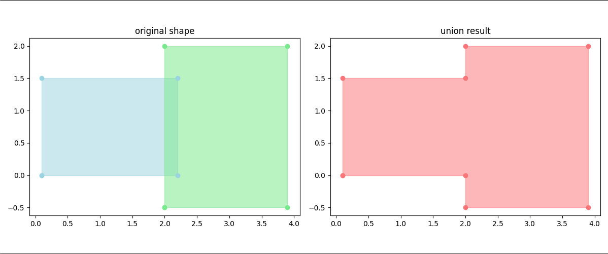
和集合
shapely_union.py
|
1 2 3 4 5 6 7 8 9 10 11 12 13 14 15 16 17 18 19 20 21 22 23 24 25 26 27 28 29 30 31 32 33 34 35 36 37 38 39 40 |
""" ShapelyとMatplotlibを使用した図形の和集合演算のサンプルコード このコードでは、2つの四角形の和集合演算を行い、結果を視覚化します。 和集合演算は、2つの図形を合わせた部分を表します。 """ from shapely.geometry import Polygon import matplotlib.pyplot as plt from shapely.plotting import plot_polygon # 1つ目の四角形を定義(時計回り) # 左下から始めて、時計回りに頂点を定義 rectangle = Polygon([(0.1, 0), (2.2, 0), (2.2, 1.5), (0.1, 1.5)]) # 2つ目の四角形を定義(時計回り) # 1つ目の四角形と一部重なるように配置 rectangle2 = Polygon([(2, -0.5), (3.9, -0.5), (3.9, 2), (2, 2)]) # 2つの四角形の和集合を計算 # union()メソッドは、2つの図形を合わせた部分を返します combined = rectangle.union(rectangle2) # 結果を視覚化するためのプロット設定 fig, (ax1, ax2) = plt.subplots(1, 2, figsize=(12, 5)) # 左側のプロット:元の図形 ax1.set_aspect('equal') ax1.set_title('original shape') plot_polygon(rectangle, ax=ax1, add_points=True, color='lightblue', alpha=0.5) plot_polygon(rectangle2, ax=ax1, add_points=True, color='lightgreen', alpha=0.5) # 右側のプロット:和集合の結果 ax2.set_aspect('equal') ax2.set_title('union result') plot_polygon(combined, ax=ax2, add_points=True, color='lightcoral', alpha=0.5) # グラフを表示 plt.tight_layout() plt.show() |
計算結果
左側に元の2つの四角形が色違いで表示され、右側に和集合の結果が表示されます。
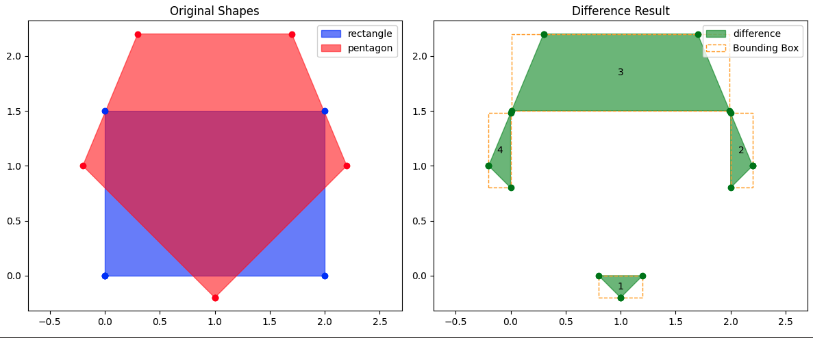
差集合
バウンディングボックスの処理も合わせて含めています。
shapely_difference.py
|
1 2 3 4 5 6 7 8 9 10 11 12 13 14 15 16 17 18 19 20 21 22 23 24 25 26 27 28 29 30 31 32 33 34 35 36 37 38 39 40 41 42 43 44 45 46 47 48 49 50 51 52 53 54 55 56 57 58 59 60 61 62 63 64 65 66 67 68 69 70 71 |
""" ShapelyとMatplotlibを使用した図形の差集合演算のサンプルコード このコードでは、四角形と五角形の差集合演算を行い、結果を視覚化します。 また、各図形のバウンディングボックスも表示します。 """ from shapely.geometry import Polygon import matplotlib.pyplot as plt from shapely.plotting import plot_polygon import matplotlib.patches as patches # 四角形の頂点を定義(時計回り) rectangle = Polygon([(0, 0), (2, 0), (2, 1.5), (0, 1.5)]) # 五角形の頂点を定義(時計回り) pentagon = Polygon([(1, -0.2), (2.2, 1), (1.7, 2.2), (0.3, 2.2), (-0.2, 1)]) # 四角形から五角形を引く(差集合演算) difference = pentagon.difference(rectangle) # 結果を視覚化するためのプロット設定 fig, (ax1, ax2) = plt.subplots(1, 2, figsize=(12, 5)) # 左側のプロット:元の図形 plot_polygon(rectangle, ax=ax1, add_points=True, color='blue', alpha=0.5, label='rectangle') plot_polygon(pentagon, ax=ax1, add_points=True, color='red', alpha=0.5, label='pentagon') ax1.set_title('Original Shapes') ax1.legend(loc='upper right') ax1.axis('equal') # 右側のプロット:差集合の結果 plot_polygon(difference, ax=ax2, add_points=True, color='green', alpha=0.5, label='difference') # バウンディングボックスの表示 if difference.geom_type == 'MultiPolygon': # 差集合が複数の多角形で構成される場合 for i, polygon in enumerate(difference.geoms): bounds = polygon.bounds # バウンディングボックスを作成 width = bounds[2] - bounds[0] height = bounds[3] - bounds[1] rect = patches.Rectangle( (bounds[0], bounds[1]), width, height, linewidth=1, edgecolor='orange', facecolor='none', linestyle='--', label=f'Bounding Box' if i == 0 else None ) ax2.add_patch(rect) # 中心点にインデックスを表示 center_x = bounds[0] + width/2 center_y = bounds[1] + height/2 ax2.text(center_x, center_y, str(i+1), horizontalalignment='center', verticalalignment='center') else: # 差集合が単一の多角形の場合 bounds = difference.bounds width = bounds[2] - bounds[0] height = bounds[3] - bounds[1] rect = patches.Rectangle( (bounds[0], bounds[1]), width, height, linewidth=1, edgecolor='orange', facecolor='none', linestyle='--', label='Bounding Box' ) ax2.add_patch(rect) ax2.set_title('Difference Result') ax2.legend(loc='upper right') ax2.axis('equal') plt.tight_layout() plt.show() |
計算結果
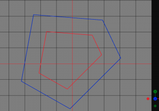
左側では青い四角形と赤い五角形が重なって表示され、右側では緑色で差集合の結果が表示されています。
外側バッファリング
shapely_outer_buffer.py
|
1 2 3 4 5 6 7 8 9 10 11 12 13 14 15 16 17 18 19 20 21 22 23 24 25 26 27 28 29 30 31 32 33 34 35 36 37 38 39 40 41 42 43 44 45 46 47 48 49 50 51 52 |
""" ShapelyとMatplotlibを使用した外側バッファリング(Outer Buffer)のサンプルコード このコードでは、多角形に対して外側バッファリングを適用し、結果を視覚化します。 """ from shapely.geometry import Polygon import matplotlib.pyplot as plt from shapely.plotting import plot_polygon from shapely.geometry import JOIN_STYLE # 複雑な形状の多角形を作成 polygon = Polygon([ (0, 0), (2, 0), (2, 1), (3, 1), (3, 2), (2, 2), (2, 3), (1, 3), (1, 2), (0, 2), (0, 1), (1, 1), (0, 0) ]) # 外側バッファリングを適用 buffer_outer = polygon.buffer(0.5, join_style=JOIN_STYLE.mitre) # 結果を視覚化 fig, (ax1, ax2) = plt.subplots(1, 2, figsize=(12, 5)) # 左側:元の多角形 plot_polygon( polygon, ax=ax1, add_points=True, color='blue', alpha=0.5, label='Original' ) ax1.set_title('Original Polygon') ax1.legend() ax1.axis('equal') # 右側:外側バッファリング plot_polygon( polygon, ax=ax2, add_points=True, color='blue', alpha=0.5, label='Original' ) plot_polygon( buffer_outer, ax=ax2, add_points=True, color='red', alpha=0.3, label='Outer Buffer' ) ax2.set_title('Outer Buffer') ax2.legend() ax2.axis('equal') # 面積の変化を表示 print(f"Original Area: {polygon.area:.2f}") print(f"Outer Buffer Area: {buffer_outer.area:.2f}") print(f"Area Increase: {(buffer_outer.area - polygon.area):.2f}") plt.tight_layout() plt.show() |
計算結果
内側に元の青い図形が表示され、外側に赤色でバッファリング後の結果が表示されています。
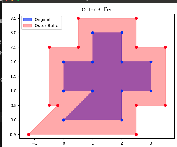
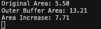
面積もターミナルに表示されます。
内側バッファリング
shapely_inner_buffer.py
|
1 2 3 4 5 6 7 8 9 10 11 12 13 14 15 16 17 18 19 20 21 22 23 24 25 26 27 28 29 30 31 32 33 34 35 36 37 38 39 40 41 42 43 44 45 46 47 48 49 50 51 52 |
""" ShapelyとMatplotlibを使用した内側バッファリング(Inner Buffer)のサンプルコード このコードでは、多角形に対して内側バッファリングを適用し、結果を視覚化します。 """ from shapely.geometry import Polygon import matplotlib.pyplot as plt from shapely.plotting import plot_polygon from shapely.geometry import JOIN_STYLE # 複雑な形状の多角形を作成 polygon = Polygon([ (0, 0), (2, 0), (2, 1), (3, 1), (3, 2), (2, 2), (2, 3), (1, 3), (1, 2), (0, 2), (0, 1), (1, 1), (0, 0) ]) # 内側バッファリングを適用(負の値) buffer_inner = polygon.buffer(-0.1, join_style=JOIN_STYLE.mitre) # 結果を視覚化 fig, (ax1, ax2) = plt.subplots(1, 2, figsize=(12, 5)) # 左側:元の多角形 plot_polygon( polygon, ax=ax1, add_points=True, color='blue', alpha=0.5, label='Original' ) ax1.set_title('Original Polygon') ax1.legend() ax1.axis('equal') # 右側:内側バッファリング plot_polygon( polygon, ax=ax2, add_points=True, color='blue', alpha=0.5, label='Original' ) plot_polygon( buffer_inner, ax=ax2, add_points=True, color='green', alpha=0.3, label='Inner Buffer' ) ax2.set_title('Inner Buffer') ax2.legend() ax2.axis('equal') # 面積の変化を表示 print(f"Original Area: {polygon.area:.2f}") print(f"Inner Buffer Area: {buffer_inner.area:.2f}") print(f"Area Decrease: {(polygon.area - buffer_inner.area):.2f}") plt.tight_layout() plt.show() |
外側には元の青い図形が表示され、内側に緑色でバッファリング後の結果が表示されています。
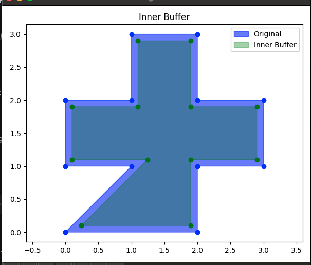
面積もターミナルに表示されます。
まとめ
今回Shapelyについて調べてみましたが、便利だと思いました。引き続き調査を続けたいと思います。
AMDlabでは、開発に力を貸していただけるエンジニアさんを大募集しております。
少しでもご興味をお持ちいただけましたら、カジュアルにお話するだけでも大丈夫ですのでお気軽にご連絡ください!
中途求人ページ: https://www.amd-lab.com/recruit-list/mid-career
カジュアル面談がエントリーフォームからできるようになりました。
採用種別を「カジュアル面談(オンライン)」にして必要事項を記載の上送信してください!
エントリーフォーム: https://www.amd-lab.com/entry


COMMENTS